Acoustic ecology - studying environments through sound
1 Accessing the assignment
Please navigate to the assignment Acoustic in
the ConBio
SP2023 workspace. In the Files pane (typically, bottom
right-hand corner), you will find an R script that you can use to follow
along with this tutorial called Acoustic.R.
Recall that:
- You can use
Tools–>Global options–>Code–> clickSoft-wrap R source filesto get word wrap enabled forRscripts. - You need to highlight (or place your cursor on a line) and run a line (or lines) of code to execute commands.
- You can tell that the code has been executed when it is echoed (printed out) in the console.
2 Overview
In this tutorial, we’ll take a look at sound data collected at the Bernard Field Station.
In this tutorial, you will learn:
- what are different ways to interact with sound data in
R? - how can we visualize sound data using spectrograms?
- how can we calculate indices of acoustic diversity?
3 A brief description of sound
When we vocalize, we are making vibrations that move through the air like a wave. Microphones detect these vibrations. These vibrations are then recorded into numbers which can be processed by computers. It turns out that we can get quite a bit of information from these numbers.
Let’s start by loading the packages that we will need.
### Loading packages
library(seewave)
library(tuneR)
library(dplyr)
library(readr)
3.1 Waveforms
Let’s pull in one of the recorded files from the BFS. You can play
the recording below. NOTE: Make sure that you use the
code in the Acoustic.R file (or the code in its entirety at
the bottom of this tutorial page) because the sound recording is in a
different location on posit.cloud than what is shown
here!
Now, let’s visualize this recording using an oscillogram. The output
from the function oscillo shows how how the amplitude (or
loudness) changes over the whole recording. We’re going to focus on
visualizing the recording from 1:01 to 1:05
## Read in the sound data
BFS_am_1 <-tuneR::readWave('20220313_063000.WAV')
## Show the oscillogram
## which is a plot of amplitude over time
## We'll focus on the first minute of the recording
oscillo(BFS_am_1, from = 0, to = 60, fastdisp=TRUE)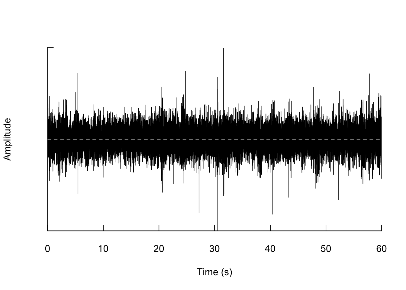
One thing to note is that these data were recorded at a frequency of 48,000 records per second. So even though each sound file is only 5 minutes long, it has a total of 14,400,000 data points! (This is equal to 5 minutes * 60 seconds / minute * 48000 records/second.)
3.2 Spectrogram
Another way that we can visualize sound is to use the fact that sound has the property of frequency (pitch) at particular times. We can also include amplitude (loudness) as a color. A spectrogram let’s us display all three elements of an acoustic signal: its time/duration, the frequency (pitch) of the sound, and the loudness of the sound at each frequency (pitch).
We see that the frequencies in this sound recording are mostly located from 0 to 5000 Hz (or 5 kHz).
## Use spectro to display the spectogram of this data
spectro(BFS_am_1, fastdisp=TRUE)
4 Soundscape indices
From observational data of species, we can calculate metrics such as species richness, Shannon’s index, etc. Similarly, from sound data, we can calculate metrics of acoustic complexity, which theoretically should be related to the overall biodiversity of vocalizing animals.
First, let’s now also read in an evening recording.
## Read in the sound data for the evening
BFS_pm_1 <-tuneR::readWave('20220313_205000.WAV')
Here, we will use the function ACI to calculate the
acoustic complexity of a morning versus evening recording from the
BFS.
ACI(BFS_am_1)## [1] 155.0816ACI(BFS_pm_1)## [1] 150.6235 Processed data: Species richness
In addition to using numeric metrics such as ACI to
calculate the acoustic diversity of audio recordings, we can use new
computer vision models to identify (bird) species in the recordings.
This therefore gives us data that we tend to see in conservation
biology: species richness. We have and will process/ed
the raw recording data to:
- Calculate ACI for each recording;
- Identify bird vocalizations in each recording;
We have used Cornell Lab of Ornithology’s BirdNET neural network model,
which is trained on data such as identified acoustic recordings from xeno-canto. This model extracts
distinct bird vocalizations from the spectrographic representation of
each sound file. Those bird vocalizations are then pattern matched
against known bird vocalizations to generate the most likely species (of
the 3000 species supported by the model) with some probability (a.k.a.
confidence).
6 Your task
Your job is to now go forward and perform the bioacoustic analysis tutorial (next drop-down menu item.) Then, think through as groups about 3 questions that you would be interested in answering using processed acoustic data from the BFS that will span from October-November 2022 and our current data in March-April 2023. Here are some suggestions about external datasets that you can look at:
- Precipitation
- Temperature
- Time of year (
date) - BirdCast migration estimates for Los Angeles County (see the Birds in flight (nightly avg.) plot FMI)
- Habitat type in the BFS (determined by the
unit’s location) - Distance to road or edge of the BFS (determined by the
unit’s location) - … other variables that you may think of and are feasible for us to collect!
###===============================================================
### Section 3
###===============================================================
### Loading packages
library(seewave)
library(tuneR)
library(dplyr)
library(readr)
###===============================================================
### Section 3.1 - 3.2
###===============================================================
## Read in the sound data
BFS_am_1 <-tuneR::readWave('BFS_sound_2022/20220313_063000.WAV')
## Show the oscillogram
## which is a plot of amplitude over time
## We'll focus on the first minute of the recording
oscillo(BFS_am_1, from = 0, to = 60, fastdisp=TRUE)
## Use spectro to display the spectogram of this data
spectro(BFS_am_1, fastdisp=TRUE)
###===============================================================
### Section 4
###===============================================================
## Read in the sound data for the evening
BFS_pm_1 <-tuneR::readWave('BFS_sound_2022/20220313_205000.WAV')
### Morning sound recording acoustic complexity index
ACI(BFS_am_1)
### Evening sound recording acoustic complexity index
ACI(BFS_pm_1)