Bioacoustic analyses
2023-04-19
1 Accessing the assignment
Please navigate to the assignment Acoustic in
the ConBio
SP2023 workspace. In the Files pane (typically, bottom
right-hand corner), you will find an R script that you can use to follow
along with this tutorial called bioacoustic.R.
Recall that:
- You can use
Tools–>Global options–>Code–> clickSoft-wrap R source filesto get word wrap enabled forRscripts. - You need to highlight (or place your cursor on a line) and run a line (or lines) of code to execute commands.
- You can tell that the code has been executed when it is echoed (printed out) in the console.
1.1 Hypotheses
This table below shows the hypotheses for each group:
| Group Number | Hypothesis | Approach |
|---|---|---|
| 1 | There will be greater edge effects (lower species richness near edges) in the morning compared to the evening. | Multiple linear regression with interaction |
| 2 | Species richness is higher at dawn | Comparison of means |
| 3 | There will be more species richness in sites with higher tree cover. | Comparison of means |
| 4 | There will be higher ACI in the northern part of BFS (the neck), than in the more southern portion. | Comparison of means |
| 5 | ACI values vary throughout the different habitats across the BFS. | Comparison of means |
| 6 | There is higher ACI or species richness in the spring than the fall. | Comparison of means |
| 7 | There will be more species recorded closer to the pond | Linear regression |
Note: The suggested analyses are not prescriptive. If you feel that a different type of analysis is better (e.g. correlation coefficient rather than comparison of means, or correlation coefficient rather than regression, or regression rather than comparison of means), then please proceed! The table above is simply intended to help speed along the analysis.
2 Preparing data
2.1 1: Load packages
Below, we will start by loading packages that we’ll need.
### Load packages
library("ggplot2") # plotting functions
library("dplyr") # data wrangling functions
library("readr") # reading in tables, including ones online
library("mosaic") # shuffle (permute) our data
2.2 2: Read data
Next, we will pull in our data and inspect it.
### Load in dataset
soundDF <- readr::read_tsv("https://github.com/chchang47/BIOL104PO/raw/master/data/bioacousticAY22-23.tsv") # read in spreadsheet from its URL and store in soundDF

### Look at the first few rows
soundDF
## # A tibble: 151,468 × 8
## unit date time ACI SR DayNight Month season
## <chr> <date> <chr> <dbl> <dbl> <chr> <chr> <chr>
## 1 CBio4 2023-03-23 18H 0M 0S 155. 3 Night March Spring
## 2 CBio4 2023-03-23 18H 1M 0S 154. 3 Night March Spring
## 3 CBio4 2023-03-23 18H 2M 0S 151. 7 Night March Spring
## 4 CBio4 2023-03-23 18H 3M 0S 155. 3 Night March Spring
## 5 CBio4 2023-03-23 18H 4M 0S 152. 2 Night March Spring
## 6 CBio4 2023-03-23 18H 5M 0S 152. 4 Night March Spring
## 7 CBio4 2023-03-23 18H 6M 0S 159. 3 Night March Spring
## 8 CBio4 2023-03-23 18H 7M 0S 152. 2 Night March Spring
## 9 CBio4 2023-03-23 18H 8M 0S 152. 3 Night March Spring
## 10 CBio4 2023-03-23 18H 9M 0S 153. 7 Night March Spring
## # ℹ 151,458 more rows### Look at the first few rows in a spreadsheet viewer
soundDF %>% head() %>% View()We see that there are the following columns:
unit: Which AudioMoth collected the recordings- Note that each AudioMoth had a particular location, so your group may use that attribute in your analyses. I’ll show you how to do that below.
date: The date of the recordingtime: The time of the recordingACI: The Acoustic Complexity Index of the recording- In a nutshell, ACI values typically increase with more diversity of sounds.
- The calculation for ACI introduced by Pieretti et al. (2011) is based on the following observations: 1) biological sounds (like bird song) tend to show fluctuations of intensities while 2) anthropogenic sounds (like cars passing or planes flying) tend to present a very constant droning sound at a less varying intensity.
- One potential confounding factor is the role of geophony, or environmental sounds like rainfall. Sometimes geophony like a low, constant wind can present at a very constant intensity, and therefore would not influence ACI. However, patterns that have high variation could influence ACI because they may have varying intensities.
SR: The species richness in every 30 second recordingDayNight: Whether the recording occurred in the day or at nightMonth: A variable that notes if the recording was taken in October, November, March, or Aprilseason: The season of the recording (fall or spring)
Here, I am going to do two tasks. I am going to create a dummy column
of data that takes the average of the ranks of SR and
ACI to illustrate different analyses. I am also going to
create a data table that tells us different characteristics of each
AudioMoth unit to illustrate how hypotheses that have some
relationship with distance or tree cover (which would be informed by the
location of the unit) could proceed.
### Creating a data table for the 14 units
# Each row is a unit and columns 2 and 3 store
# values for different attributes about these units
unit_table <- tibble::tibble(
unit = paste("CBio",c(1:14),sep=""), # create CBio1 to CBio14 in ascending order
sitecat = c("Tree","Tree","Tree","Tree","Tree",
"Tree","Tree","Open","Open","Open",
"Open","Open","Open","Open"), # categorical site variable, like degree of tree cover
sitenum = c(1,5,8,9,4,
3,-2,-5,-1,-6,
2.5,-3.4,6.5,4.7) # numeric site variable, like distance
)View(unit_table) # take a look at this table to see if it lines up with what you expect### Creating a dummy variable for example analyses below
soundDF <- soundDF %>%
mutate(ChangVar =(rank(ACI)+ rank(SR))/2)Sometimes, data that we want to combine for analyses are separated
across different spreadsheets or data tables. How can we combine these
different data tables? Join operations (FMI
on joining two data tables) offer a way to merge data
across multiple data tables (also called data frames in R
parlance).
In this case, we want to add on the site features of the 14 AudioMoth
units to the bioacoustic data. I am going to use the
left_join operation to add on the unit characteristics
defined in unit_table above.
### Adding on the site features of the 14 AudioMoth units
soundDF <- soundDF %>%
left_join(unit_table, by=c("unit"="unit")) # Join on the data based on the value of the column unit in both data tables3 Data exploration
Below, I provide fully-worked examples of different ways of
inspecting your data and performing analyses assuming that
ChangVar is the variable of interest. In applying
this code to your own data, you will want to think about what variable
name should replace ChangVar in the commands
below. For example, you would change
tapply(soundDF$ChangVar, soundDF$sitecat, summary) to
tapply(soundDF$ResponseVariable, soundDF$sitecat, summary)
where ResponseVariable is the variable you’re
analyzing.
Let’s start with exploratory data analysis where you calculate summary statistics and visualize your variable.
### Calculate summary statistics for ChangVar
### for each sitecat
tapply(soundDF$ChangVar, soundDF$sitecat, summary) ## $Open
## Min. 1st Qu. Median Mean 3rd Qu. Max.
## 8095 47172 77256 73805 100275 149904
##
## $Tree
## Min. 1st Qu. Median Mean 3rd Qu. Max.
## 8046 52731 80302 77683 103211 151085 # use sitecat as the grouping variable
# for ChangVar and then summarize ChangVar
# for each sitecat (site characteristics)3.1 Visualization
How would I visualize the values of ChangVar? I could
use something like a histogram and color the values differently for the
categories in sitecat.
### Creating a histogram
# Instantiate a plot
p <- ggplot(soundDF, aes(x=ChangVar,fill=sitecat))
# Add on a histogram
p <- p + geom_histogram()
# Change the axis labels
p <- p + labs(x="Mean of ranks",y="Frequency")
# Change the plot appearance
p <- p + theme_minimal()
# Display the final plot
p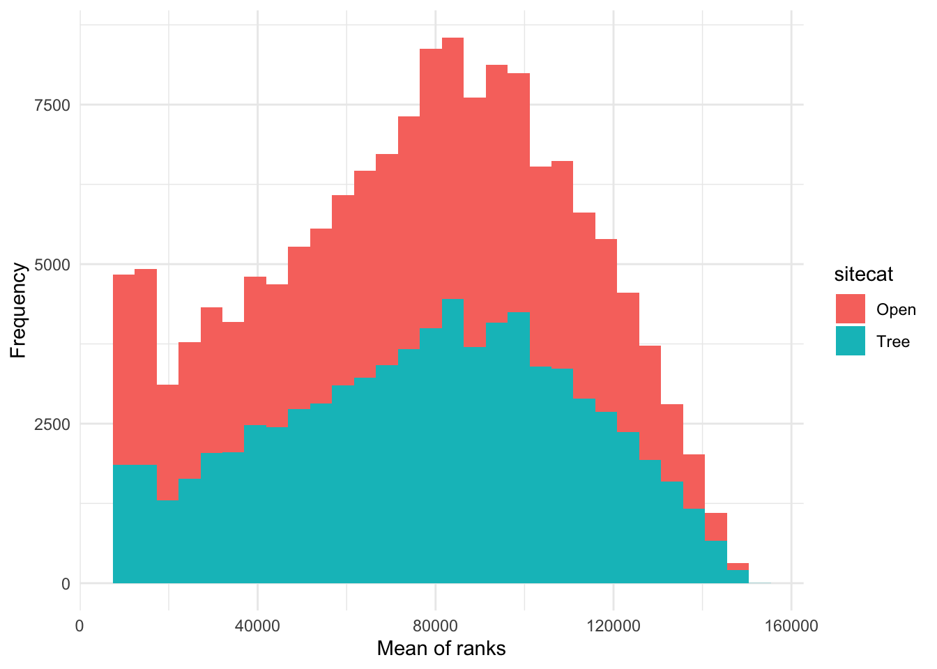
Alternatively, I could create a boxplot to visualize the distribution
of values in ChangVar with two boxplots for each value of
sitecat. Note that notch=TRUE means that there
will be a 95% confidence interval added to the median of the
boxplot.
### Creating a boxplot
# Instantiate a plot
p <- ggplot(soundDF, aes(x=sitecat, y=ChangVar, fill=sitecat))
# Add on a boxplot
p <- p + geom_boxplot(notch=TRUE)
# Change the axis labels
p <- p + labs(x="Site cat",y="Ranks")
# Change the plot appearance
p <- p + theme_classic()
# Display the final plot
p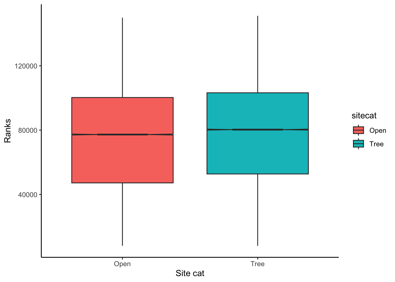
Finally, if I am interested in the relationship between two or more numeric variables, I can use a scatterplot to visualize each pair of data.
### Creating a scatterplot
# Instantiate a plot
p <- ggplot(soundDF, aes(x=sitenum, y=ChangVar, color=sitecat))
# Add on a scatterplot
p <- p + geom_point()
# Change the axis labels
p <- p + labs(x="Site num",y="Ranks")
# Change the plot appearance
p <- p + theme_bw()
# Display the final plot
p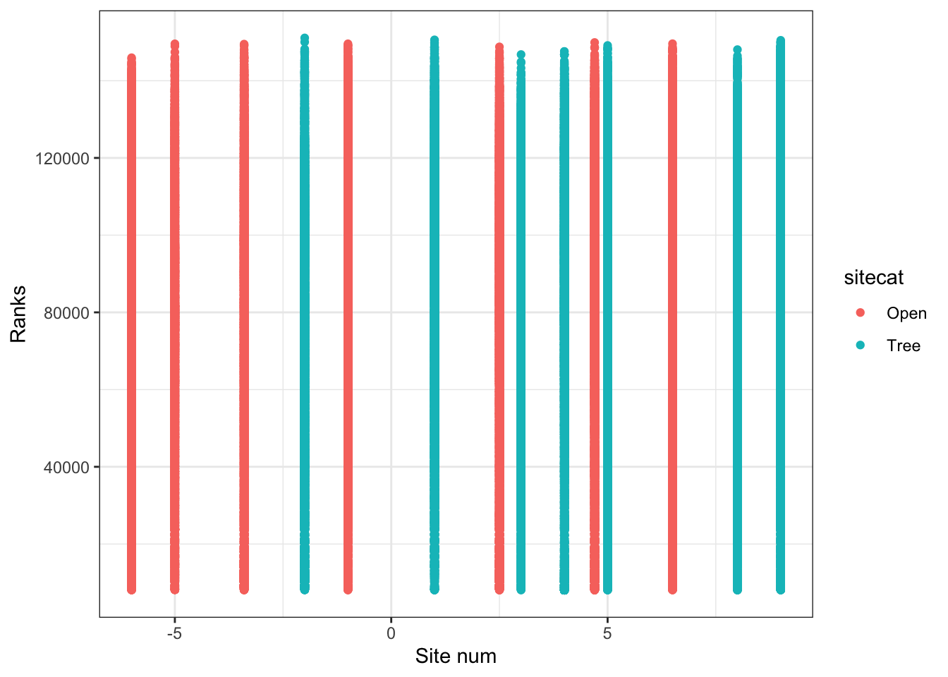
4 Statistical analysis
The code below shows you how to do different types of analyses.
4.1 1: Calculating differences in means
Let’s say I am interested in determining
if Tree sites tend to have higher ChangVar ranks. This
sounds like I want to see if there is a clear difference in the mean
values of ChangVar for the Tree vs. Open sites. We can
start by calculating the mean difference we observe.
mean( ChangVar ~ sitecat, data = soundDF , na.rm=T) # show mean ChangVar values for the Big and Open sites, removing missing data## Open Tree
## 73805.17 77682.87obs_diff <- diff( mean( ChangVar ~ sitecat, data = soundDF , na.rm=T)) # calculate the difference between the means and store in a variable called "obs_diff"
obs_diff # display the value of obs_diff## Tree
## 3877.701OK, so the mean difference in mean values between Big and Open sites is 3877.7. Is this difference meaningful though? We can test that by specifying an opposing null hypothesis.
In this case, our null hypothesis would be that there is no
difference in ChangVar across sitecat.
Logically, if there is a meaningful difference, then if we shuffle our data around, that should lead to different results than what we see. That is one way to simulate statistics to test the null hypothesis. And specifically, in this case, we would expect to see our observed difference is much larger (or much smaller) than most of the simulated values.
Let’s shuffle the data 1000 times according to the null hypothesis
(where sitecat doesn’t matter for influencing
ChangVar) and see what that means for the distribution of
mean ChangVar differences between Tree and Open sites.
### Create random differences by shuffling the data
randomizing_diffs <- do(1000) * diff( mean( ChangVar ~ shuffle(sitecat),na.rm=T, data = soundDF) ) # calculate the mean in ChangVar when we're shuffling the site characteristics around 1000 times
# Clean up our shuffled data
names(randomizing_diffs)[1] <- "DiffMeans" # change the name of the variable
# View first few rows of data
head(randomizing_diffs)## DiffMeans
## 1 111.65401
## 2 45.55392
## 3 104.20120
## 4 172.06861
## 5 -85.71986
## 6 -72.35591Now we can visualize the distribution of simulated differences in the
mean values of ChangVar at the Big and Open sites versus
our observed difference in means. Note that the observed difference was
less than 0. So in this case, more extreme data would be more extremely
small. Thus, we need to use <= below in the
fill = ~ part of the command.
gf_histogram(~ DiffMeans, fill = ~ (DiffMeans <= obs_diff),
data = randomizing_diffs,
xlab="Difference in mean ChangVar under null",
ylab="Count")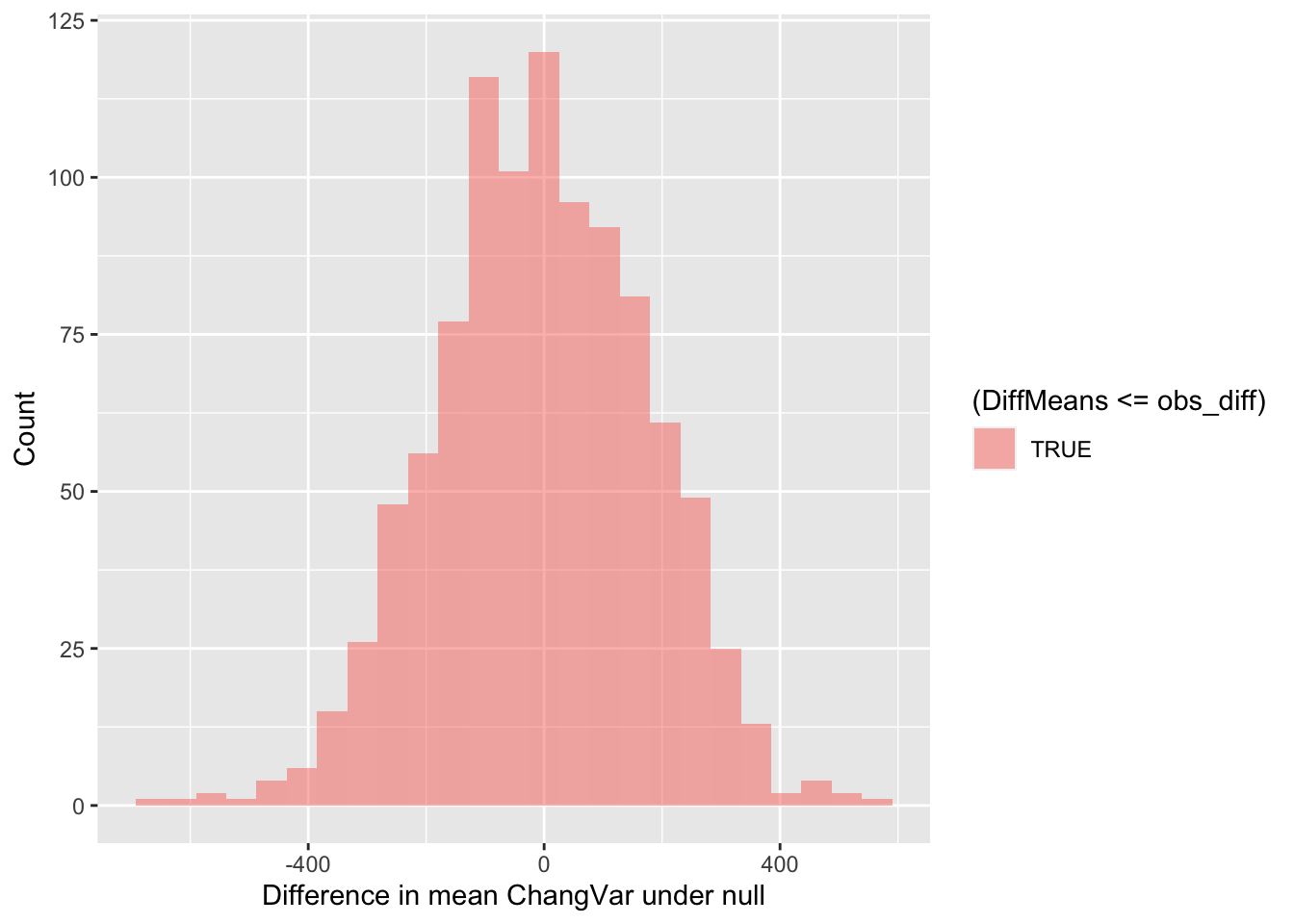
In the end, how many of the simulated mean differences were more extreme than the value we observed? This is a probability value or a p-value for short.
# What proportion of simulated values were larger than our observed difference
prop( ~ DiffMeans <= obs_diff, data = randomizing_diffs) # ~0.0 was the observed difference value - see obs_diff## prop_TRUE
## 1Wow! Our observation was really extreme. The p-value we’ve calculated is 0. The simulated mean differences were never more extreme(ly small) than our observed difference in means. Based on this value, if we were using the conventional \(p\)-value (probability value) of 0.05, we would conclude that because this simulated \(p\)-value <<< 0.05, that we can reject the null hypothesis.
4.1.1 Statistical test
Alternatively, we can run a test. If we are concerned about potential violations to normality, we can use a non-parametric test to compare means.
# Statistical test - comparing means between two categories
t.test(ChangVar ~ sitecat, data=soundDF)##
## Welch Two Sample t-test
##
## data: ChangVar by sitecat
## t = -22.053, df = 151380, p-value < 2.2e-16
## alternative hypothesis: true difference in means is not equal to 0
## 95 percent confidence interval:
## -4222.333 -3533.069
## sample estimates:
## mean in group Open mean in group Tree
## 73805.17 77682.87# Statistical test - non-parametric - comparing means between two categories
wilcox.test(ChangVar ~ sitecat, data=soundDF)##
## Wilcoxon rank sum test with continuity correction
##
## data: ChangVar by sitecat
## W = 2.698e+09, p-value < 2.2e-16
## alternative hypothesis: true location shift is not equal to 0If we are comparing a numeric value across more than three categories in the data, we can either use an ANOVA or a non-parametric test (robust to violating assumptions about the distribution of your data and the errors of your model) such as a Kruskal-Wallis test.
# Run the ANOVA test
anova_test <- aov(ChangVar ~ Month, data=soundDF)
# See the outputs
summary(anova_test)
# Run the non-parametric Kruskal-Wallis test
kw_test <- kruskal.test(ChangVar ~ Month, data=soundDF)
# See the outputs
kw_test4.2 Calculating correlation coefficients
Now let’s say that you’re interested in comparing
ChangVar, a numeric variable, against another numeric
variable like sitenum. One way to do that is to calculate a
confidence interval for their correlation coefficient.
How would I determine if there is a non-zero correlation between two variables or that two variables are positively correlated? I can again start by calculating the observed correlation coefficient for the data.
### Calculate observed correlation
obs_cor <- cor(ChangVar ~ sitenum, data=soundDF, use="complete.obs") # store observed correlation in obs_cor of ChangVar vs sitenum
obs_cor # print out value## [1] 0.05162087Let’s say that I’m interested in determining if ChangVar
is actually positively correlated with sitenum. We can test
this against the opposing null hypothesis. Our null hypothesis could be
that the correlation coefficient is actually 0.
As before though, how do I know that my correlation coefficient of 0 is significantly different from 0? We can tackle this question by simulating a ton of correlation coefficient values from our data by shuffling it!
In this case, the shuffling here lets us estimate the variation in the correlation coefficient given our data. So we are curious now if the distribution of simulated values does or does not include 0 (that is, is it clearly \(< 0\) or \(> 0\)?).
### Calculate correlation coefs for shuffled data
randomizing_cor <- do(1000) * cor(ChangVar ~ sitenum,
data = resample(soundDF),
use="complete.obs")
# Shuffle the data 1000 times
# Calculate the correlation coefficient each time
# By correlating ChangVar to sitenum from the
# data table soundDFWhat are the distribution of correlation coefficients that we see when we shuffle our data?
quantiles_cor <- qdata( ~ cor, p = c(0.025, 0.975), data=randomizing_cor) # calculate the 2.5% and 97.5% quantiles in our simulated correlation coefficient data (note that 97.5-2.5 = 95!)
quantiles_cor # display the quantiles## 2.5% 97.5%
## 0.04678683 0.05627252The values above give us a 95% confidence interval estimate for our correlation coefficient!
Do we clearly see that our correlation coefficient distribution does or doesn’t include 0?
gf_histogram(~ cor,
data = randomizing_cor,
xlab="Simulated correlation coefficients",
ylab="Count")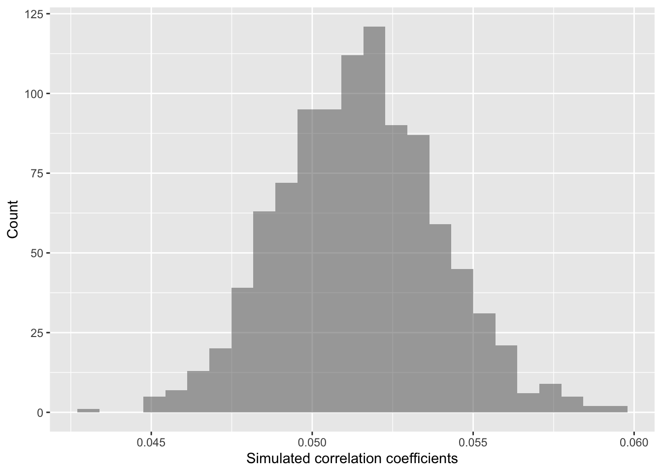
In this case, our simulated correlation coefficient includes 0 in its
95% simulated confidence interval. We can also see this in the plot. So
given these data, we cannot reject the null hypothesis. There is not
sufficiently strong data that the mean ranks in ChangVar
associate with site characteristics in sitenum in any clear
way.
4.2.1 Statistical test
We can also use a statistical test here rather than a
permutation-based analysis. If we wanted to run a test of the
correlation coefficient, we could use the cor.test function
in R. If we are concerned about violations of normality, we
can also used non-parametric, rank-based tests.
cor.test(ChangVar~sitenum, data=soundDF, method="spearman")##
## Spearman's rank correlation rho
##
## data: ChangVar and sitenum
## S = 5.5471e+14, p-value < 2.2e-16
## alternative hypothesis: true rho is not equal to 0
## sample estimates:
## rho
## 0.042245514.3 Linear regression
In the context of these data, it is not as obvious how a linear regression would be 1) appropriate (e.g. comparing across categories is arguably better done with a comparison of means) or 2) more insightful than the correlation analysis above.
However, for completeness I show how we could fit a regression model.
### Regression model for ACI
aci_mod <- lm(ACI ~ sitenum, data=soundDF)
summary(aci_mod)##
## Call:
## lm(formula = ACI ~ sitenum, data = soundDF)
##
## Residuals:
## Min 1Q Median 3Q Max
## -12.054 -3.452 -2.082 0.690 179.123
##
## Coefficients:
## Estimate Std. Error t value Pr(>|t|)
## (Intercept) 1.543e+02 2.002e-02 7704.40 <2e-16 ***
## sitenum 9.650e-02 4.041e-03 23.88 <2e-16 ***
## ---
## Signif. codes: 0 '***' 0.001 '**' 0.01 '*' 0.05 '.' 0.1 ' ' 1
##
## Residual standard error: 7.237 on 151466 degrees of freedom
## Multiple R-squared: 0.003751, Adjusted R-squared: 0.003744
## F-statistic: 570.2 on 1 and 151466 DF, p-value: < 2.2e-16If one wanted to analyze species richness as a response variable, we
would need to use an alternative to lm (ordinary least
squares regression) and use a glm (generalized linear
model). Species richness values are integers (whole
numbers). That means that they are better modeled using a Poisson
process, which lets us think about the rates of seeing integer numbers
(e.g. number of days before another big rain event, number of fish
swimming down a stretch of river).
### Regression model for species richness
# Need to use a generalized linear model
# Because species richness is an integer value
# So we have to use poisson-distributed errors
sr_mod <- glm(SR~sitenum, data=soundDF,family=poisson)
summary(sr_mod)##
## Call:
## glm(formula = SR ~ sitenum, family = poisson, data = soundDF)
##
## Deviance Residuals:
## Min 1Q Median 3Q Max
## -2.2689 -1.1181 -0.3616 0.8314 6.2756
##
## Coefficients:
## Estimate Std. Error z value Pr(>|z|)
## (Intercept) 0.9375071 0.0017326 541.093 <2e-16 ***
## sitenum 0.0008825 0.0003493 2.526 0.0115 *
## ---
## Signif. codes: 0 '***' 0.001 '**' 0.01 '*' 0.05 '.' 0.1 ' ' 1
##
## (Dispersion parameter for poisson family taken to be 1)
##
## Null deviance: 339016 on 151467 degrees of freedom
## Residual deviance: 339010 on 151466 degrees of freedom
## AIC: 682210
##
## Number of Fisher Scoring iterations: 54.3.1 Multiple linear regression with an interaction effect
Below, I will show you how you can specify an interaction
effect (more
involved explainer here with an R example) in a
multiple linear regression, or a regression model which has more than
one predictor variable.
### Specify a generalized linear regression model for species richness with an interaction term
sr_int_mod <- glm(SR~sitenum + sitecat + sitenum*sitecat, data=soundDF, family=poisson)
### See the outputs
summary(sr_int_mod)##
## Call:
## glm(formula = SR ~ sitenum + sitecat + sitenum * sitecat, family = poisson,
## data = soundDF)
##
## Deviance Residuals:
## Min 1Q Median 3Q Max
## -2.2850 -1.1259 -0.3598 0.8356 6.2945
##
## Coefficients:
## Estimate Std. Error z value Pr(>|z|)
## (Intercept) 0.9402080 0.0022701 414.173 < 2e-16 ***
## sitenum 0.0029793 0.0005076 5.869 4.38e-09 ***
## sitecatTree 0.0053173 0.0040857 1.301 0.193
## sitenum:sitecatTree -0.0046273 0.0008098 -5.714 1.10e-08 ***
## ---
## Signif. codes: 0 '***' 0.001 '**' 0.01 '*' 0.05 '.' 0.1 ' ' 1
##
## (Dispersion parameter for poisson family taken to be 1)
##
## Null deviance: 339016 on 151467 degrees of freedom
## Residual deviance: 338975 on 151464 degrees of freedom
## AIC: 682179
##
## Number of Fisher Scoring iterations: 5### Specify a linear regression model for ACI with an interaction term
ACI_int_mod <- lm(ACI~sitenum + sitecat + sitenum*sitecat, data=soundDF)
### See the outputs
summary(ACI_int_mod)##
## Call:
## lm(formula = ACI ~ sitenum + sitecat + sitenum * sitecat, data = soundDF)
##
## Residuals:
## Min 1Q Median 3Q Max
## -12.396 -3.449 -2.079 0.691 178.851
##
## Coefficients:
## Estimate Std. Error t value Pr(>|t|)
## (Intercept) 1.540e+02 2.627e-02 5862.075 < 2e-16 ***
## sitenum 2.750e-02 5.875e-03 4.680 2.87e-06 ***
## sitecatTree 4.256e-01 4.735e-02 8.988 < 2e-16 ***
## sitenum:sitecatTree 9.231e-02 9.369e-03 9.853 < 2e-16 ***
## ---
## Signif. codes: 0 '***' 0.001 '**' 0.01 '*' 0.05 '.' 0.1 ' ' 1
##
## Residual standard error: 7.229 on 151464 degrees of freedom
## Multiple R-squared: 0.005899, Adjusted R-squared: 0.005879
## F-statistic: 299.6 on 3 and 151464 DF, p-value: < 2.2e-165 Your task
Each of your groups is required to submit 3 hypotheses by the end of this lab. Please confer with your groups on possible hypotheses that you can explore with these data. Note that a hypothesis is a falsifiable statement–e.g., “Bird richness is higher near candy shops than cat shelters,” rather than “Where are birds located? Are they near candy shops or cat shelters or somewhere else?”
6 Code in entirety
The segment below can be directly copied and pasted into the code editor in RStudio Cloud.
###=========================================
### 2: Load packages
###=========================================
library("ggplot2") # plotting functions
library("dplyr") # data wrangling functions
library("readr") # reading in tables, including ones online
library("mosaic") # shuffle (permute) our data
###=========================================
### 2: Preparing data
###=========================================
### Load in dataset
soundDF <- readr::read_tsv("https://github.com/chchang47/BIOL104PO/raw/master/data/bioacousticAY22-23.tsv") # read in spreadsheet from its URL and store in soundDF
### Look at the first few rows
soundDF
### Look at the first few rows in a spreadsheet viewer
soundDF %>% head() %>% View()
### Creating a data table for the 14 units
  # Each row is a unit and columns 2 and 3 store
  # values for different attributes about these units
unit_table <- tibble::tibble(
  unit = paste("CBio",c(1:14),sep=""), # create CBio1 to CBio14 in ascending order
  sitecat = c("Tree","Tree","Tree","Tree","Tree",
              "Tree","Tree","Open","Open","Open",
              "Open","Open","Open","Open"), # categorical site variable, like degree of tree cover
  sitenum = c(1,5,8,9,4,
              3,-2,-5,-1,-6,
              2.5,-3.4,6.5,4.7) # numeric site variable, like distance
)
View(unit_table) # take a look at this table to see if it lines up with what you expect
### Creating a dummy variable for example analyses below
soundDF <- soundDF %>%
  mutate(ChangVar =(rank(ACI)+ rank(SR))/2)
### Adding on the site features of the 14 AudioMoth units
soundDF <- soundDF %>%
  left_join(unit_table, by=c("unit"="unit")) # Join on the data based on the value of the column unit in both data tables
###=========================================
### 3: Data exploration
###=========================================
### Calculate summary statistics for ChangVar
### for each sitecat
tapply(soundDF$ChangVar, soundDF$sitecat, summary)
### Creating a histogram
  # Instantiate a plot
p <- ggplot(soundDF, aes(x=ChangVar,fill=sitecat))
  # Add on a histogram
p <- p + geom_histogram()
  # Change the axis labels
p <- p + labs(x="Mean of ranks",y="Frequency")
  # Change the plot appearance
p <- p + theme_minimal()
  # Display the final plot
p
### Creating a boxplot
# Instantiate a plot
p <- ggplot(soundDF, aes(x=sitecat, y=ChangVar, fill=sitecat))
# Add on a boxplot
p <- p + geom_boxplot()
# Change the axis labels
p <- p + labs(x="Site cat",y="Ranks")
# Change the plot appearance
p <- p + theme_classic()
# Display the final plot
p
### Creating a scatterplot
  # Instantiate a plot
p <- ggplot(soundDF, aes(x=sitenum, y=ChangVar, color=sitecat))
  # Add on a scatterplot
p <- p + geom_point()
  # Change the axis labels
p <- p + labs(x="Site num",y="Ranks")
  # Change the plot appearance
p <- p + theme_bw()
  # Display the final plot
p
###=========================================
### 4: Statistical analysis
###=========================================
###*************
###* 4.1: Difference in means
###*************
mean( ChangVar ~ sitecat, data = soundDF , na.rm=T) # show mean ChangVar values for the Big and Open sites, removing missing data
obs_diff <- diff( mean( ChangVar ~ sitecat, data = soundDF , na.rm=T)) # calculate the difference between the means and store in a variable called "obs_diff"
obs_diff # display the value of obs_diff
### Create random differences by shuffling the data
randomizing_diffs <- do(1000) * diff( mean( ChangVar ~ shuffle(sitecat),na.rm=T, data = soundDF) ) # calculate the mean in ChangVar when we're shuffling the site characteristics around 1000 times
  # Clean up our shuffled data
names(randomizing_diffs)[1] <- "DiffMeans" # change the name of the variable

# View first few rows of data
head(randomizing_diffs)
# Plot the simulated vs. observed value
# Think about the direction in fill! <= or =>
gf_histogram(~ DiffMeans, fill = ~ (DiffMeans <= obs_diff),
             data = randomizing_diffs,
             xlab="Difference in mean ChangVar under null",
             ylab="Count")
# What proportion of simulated values were larger than our observed difference
prop( ~ DiffMeans <= obs_diff, data = randomizing_diffs) # ~0.0 was the observed difference value - see obs_diff
# Statistical test - comparing means between two categories
t.test(ChangVar ~ sitecat, data=soundDF)
# Statistical test - non-parametric - comparing means between two categories
wilcox.test(ChangVar ~ sitecat, data=soundDF)
# Run the ANOVA test
anova_test <- aov(ChangVar ~ Month, data=soundDF)
# See the outputs
summary(anova_test)

# Run the non-parametric Kruskal-Wallis test
kw_test <- kruskal.test(ChangVar ~ Month, data=soundDF)
# See the outputs
kw_test
###*************
###* 4.2: Correlation coefficients
###*************
### Calculate observed correlation
obs_cor <- cor(ChangVar ~ sitenum, data=soundDF, use="complete.obs") # store observed correlation in obs_cor of ChangVar vs sitenum
obs_cor # print out value
### Calculate correlation coefs for shuffled data
randomizing_cor <- do(1000) * cor(ChangVar ~ sitenum,
                                 data = resample(soundDF),
                                 use="complete.obs")
# Shuffle the data 1000 times
# Calculate the correlation coefficient each time
# By correlating ChangVar to sitenum from the
# data table soundDF
quantiles_cor <- qdata( ~ cor, p = c(0.025, 0.975), data=randomizing_cor) # calculate the 2.5% and 97.5% quantiles in our simulated correlation coefficient data (note that 97.5-2.5 = 95!)
quantiles_cor # display the quantiles
gf_histogram(~ cor,
             data = randomizing_cor,
             xlab="Simulated correlation coefficients",
             ylab="Count")
# Statistical test
cor.test(ChangVar~sitenum, data=soundDF, method="spearman")
### Regression models
aci_mod <- lm(ACI ~ sitenum, data=soundDF)
summary(aci_mod)
sr_mod <- glm(SR~sitenum, data=soundDF,family=poisson)
summary(sr_mod)
### Specify a generalized linear regression model for species richness with an interaction term
sr_int_mod <- glm(SR~sitenum + sitecat + sitenum*sitecat, data=soundDF, family=poisson)
### See the outputs
summary(sr_int_mod)
### Specify a linear regression model for ACI with an interaction term
ACI_int_mod <- lm(ACI~sitenum + sitecat + sitenum*sitecat, data=soundDF)
### See the outputs
summary(ACI_int_mod)